tags : Math, Causal Inference, Machine Learning, Clustering
Stats is about changing your mind under uncertainty
FAQ
Bayesian or Frequentist
- The difference is philosophical
- The statistical war is over, we no longer talk about this
- We’re more interested in how we justify our statistical procedures, whether they’re Bayesian or frequentist, which leads us to Causal Inference
- The right one to choose depends on how you want to approach your decision-making.
- Eg. If you have no default action, go Bayesian.
- Also see Bayesian Statistics: The three cultures | Hacker News
Differences
| Bayesian | Frequentist | |
|---|---|---|
| Parameter | It is a random variable. It’s perspective, no right or wrong. | It’s not a random variable. Answer is fixed and unknown, there’s one “right answer” |
| Goal | Opinions to have (prior belief) | Actions to take (default action) |
| Thinking | I have an perspective, let’s see how it changes if i add data to it | We try to figure out an evidence that convinces me to choose an action |
| Coin-Toss | It’s 50% heads for me, but 100% for you because you know already | It’s 100% either heads or tails, I just don’t know the answer |
| Jargon | credible interval, prior, posterior | confidence interval, p-value, power, significance, method quality |
Neural Networks Bayesian or Frequentist?
From a deleted reddit user: Source: I’m a machine learning engineer
“Frequentist” and “bayesian” are a categorization of ways of thinking about the meaning probability and statistics.
- A frequentist thinks in terms of analyzing a collection of data.
- A bayesian thinks in terms of quantifying ignorance.
The prototypical example is that
- frequentist would say that a probability is a frequency of occurrence in a data set
- a bayesian would say that a probability is a quantification of uncertainty that exists independently of any actual data.
The difference between the two isn’t actually important; the math is always the same, the difference is just the story you choose to tell about it.
Machine learning sometimes seems more bayesian in the sense that ML algorithms produce probabilities as outputs, and these probabilities are not frequencies of occurrence in a data set; they’re something a bit more complicated than that. But these algorithms are ultimately just mathematical models that have been fitted to actual data, so the frequentist story is also applicable. (Neural networks typically estimate fixed, single values for parameters (weights and biases)
Regular statistics are still very relevant, and people who dismiss ML as “statistics on computers” are not at all far from the mark. I use A/B testing and confidence intervals in my work all the time, and it would probably be very useful for me to know more about hypothesis testing than I currently do.
I do think that the term “bayesian” is overused and often not effective at communicating anything meaningful, and I sympathize with whoever said “a bayesian is just someone who uses bayes’ rule even when it’s inappropriate.”
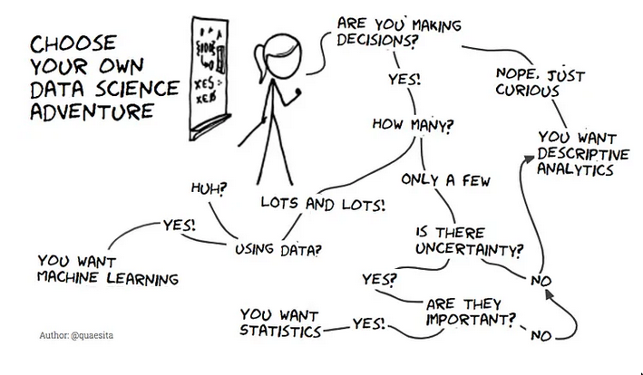
Difference between statistics and analytics
- Analytics
- We always learn something (scope of your interest is the data that’s in front)
- Analytics cares about what’s here. i.e Stick to the data and don’t go beyond it.
- When you go beyond your data, you venture into statistics
- Statics
- Sometimes we do something with the
sampleand it tells us nothing about thepopulation - It’s okay and good to learn nothing in statistics after analyzing our data/testing your hypothesis.
- Statistics cares more about what isn’t.
- Sometimes we do something with the
Rounding Numbers
It was surprising to me that I am was on the wrong side when coming to rounding numbers! Most important thing is to round in one step and to round in the last step of the calculation.
- Draw a line mentally at the point where you want to round.
- If the number next to the line is 0-4, throw away everything to the right of the line.
- If the number next to the line is 5-9, raise the digit to the left by one and throw away everything to the right of the line.
Eg. 1.2|4768 ~ 1.2 but 1.2|7432 ~ 1.3
Basics
Sample and Population
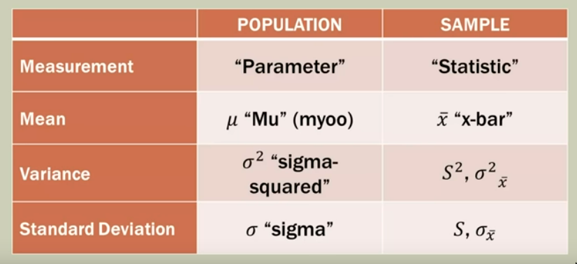 Because of this, we can see two versions of formulas, one for population and one for sample
Population
There are no set rules to apply when defining a population except knowledge, common sense, and judgment
Sample
- It’s an approximation of the population
- Always will have some error in them
- It is usually a subgroup of the population, but in a census, the whole population is the sample. The sample size is usually denoted as n and the population size as N and the sample size is always a definite number.
-
Good and bad samples
A good sample is a smaller group that is representative of the population, all valid samples are chosen through probability means. Following are some ways to collect samples, ordered by preference:
-
Random Samples
Random doesn’t mean unplanned; even collecting random samples needs proper planning. For this, you need a list and some way to select random subjects from the list for your sample.
-
Systematic Samples
Best explained through an example, Standing outside the grocery store all day, you survey every 40th person. That is a systematic sample with k=40.
-
Cluster Samples
This one makes a big assumption, that the individuals in each cluster are representative of the whole population. A cluster sample cannot be analyzed in all the same ways as random or systematic samples. You subdivide the population into a large number of subunits(clusters) and then construct random samples from the clusters.
-
Stratified Samples
This needs analyzing what data you’ll be working with, if you can identify subgroups(strata) that have something in common related to what you’re trying to study, you want to ensure that you have the same mix of those groups as the population. Eg. 45% Girls and 55% Boys in a school, If you’re taking samples of 400, it should be 45% x 400 and 55% x 400, each mini sample should be constructed using other random sampling methods.
-
Census
A census sample contains every member of the population.
-
Statistics types
Descriptive Statistics
- Summarizing and presenting the data that was measured
- Can be done for both
quantitativeandcategoricaldata - statistic
- a statement of Descriptive stats
- a numerical summary of a
sample
Inferential Statistics
- Making statements about the population based on measurements of a smaller sample.
INFERENCE = DATA + ASSUMPTIONS, i.e statistics does not give you truth. The way to “require less data” is to make bigger assumptions.- An
assumptionis not a fact, it’s some nonsense you make up precisely because you’ve got gaping holes in your knowledge. But they’re important. - parameter
- a statement of Inferential stats
- a numerical summary of a
population
Errors
In stats, errors are not like programing errors but are the discrepancy between your findings and reality.
Sampling error
These are part of the sampling process, cannot be eliminated can be minimized by increasing the sample size
Non-sampling error
When you mess up in collecting data/analyzing data etc.
Data and experiments
Variables
Variables are the question and data points are the answers. Eg. birth weight is the variable and 5Kg will be the data point. sometimes variable type is also called data type.
In either observational study or experimental study there are two variables:
- Explanatory variables/factors: Suspected causes
- Response variables: Suspected effects/results
-
Explanatory variables that make the results/response variables questionable:
-
Lurking variables: A hidden variable that isn’t measured but affects the outcome. A careful randomized experimental study can get rid of these.
-
Confounding variables: You know what they are, but you cannot untangle their effect from what you actually wanted. Try to rule these out if possible before experimentation.
-
-
Quantitative and Qualitative
-
Quantitative
Numeric, sometimes it’s hard to differentiate between discrete and contd. but it’s important to identify the difference when you need to graph them
- Discrete: how many
- Contd. : how much
-
Qualitative/Categorical
non-numeric
-
Gathering data
-
Observational study
A retrospective study. Lurking variables are the reason an obs study can never establish cause/causation, no matter how strong of an association do you find.
-
Experiment
Here we can manipulate the explanatory variables, each level of the assigned explanatory variable is known as a treatment. If we do have a randomized experiment, we can prove causation. Eg. Doing a study by giving your 3 children different toys, the explanatory variable is
toy, and treatments are the different toys.
Basics of designing experiments
Completely Randomized Design
Randomly assign members to the various treatment groups, this is called randomization
Randomized Block Design
When there is a confounding variable that you can detect, before conducting the experiment divide subjects into blocks according to that variable, then randomize within each block. This variable is called the blocking variable. i.e confounding variable became the blocking variable here.
“Block what you can, randomize what you cannot”
Matched pairs
Type of randomized block design where each block contains two identical subjects without any fear of lurking variables. (Eg. twins) another special type is matching experimental results with itself (eg. delta)
Control groups and placebo
When doing experiments involving the placebo effect, the group that gets the placebo is called the control group
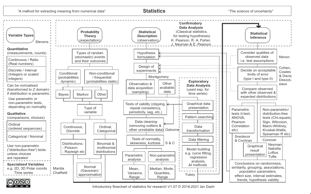
Distributions
Meta
- Distributions themselves are not specific to either frequentist or Bayesian statistics
- Frequentist statistics uses distributions to model the frequency of data and outcomes.
- Bayesian statistics uses distributions to model the probability and uncertainty of parameters.
Frequency Distribution
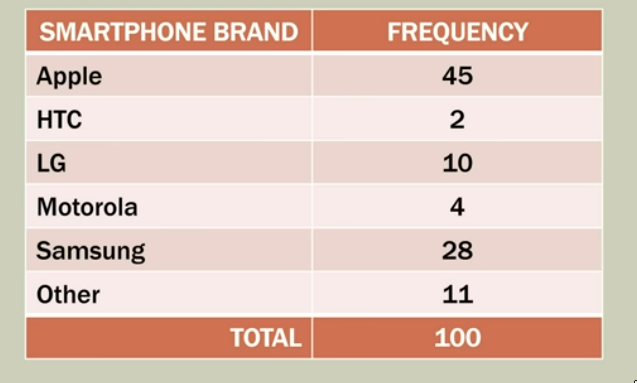
Descriptive Stats
3M (Center of Data)
- Mean, Median and Mode
- Measure the
centerof the data
Mean
-
Arithmetic Mean/Sample mean
- Useful for additive processes
-
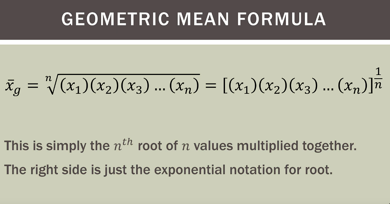
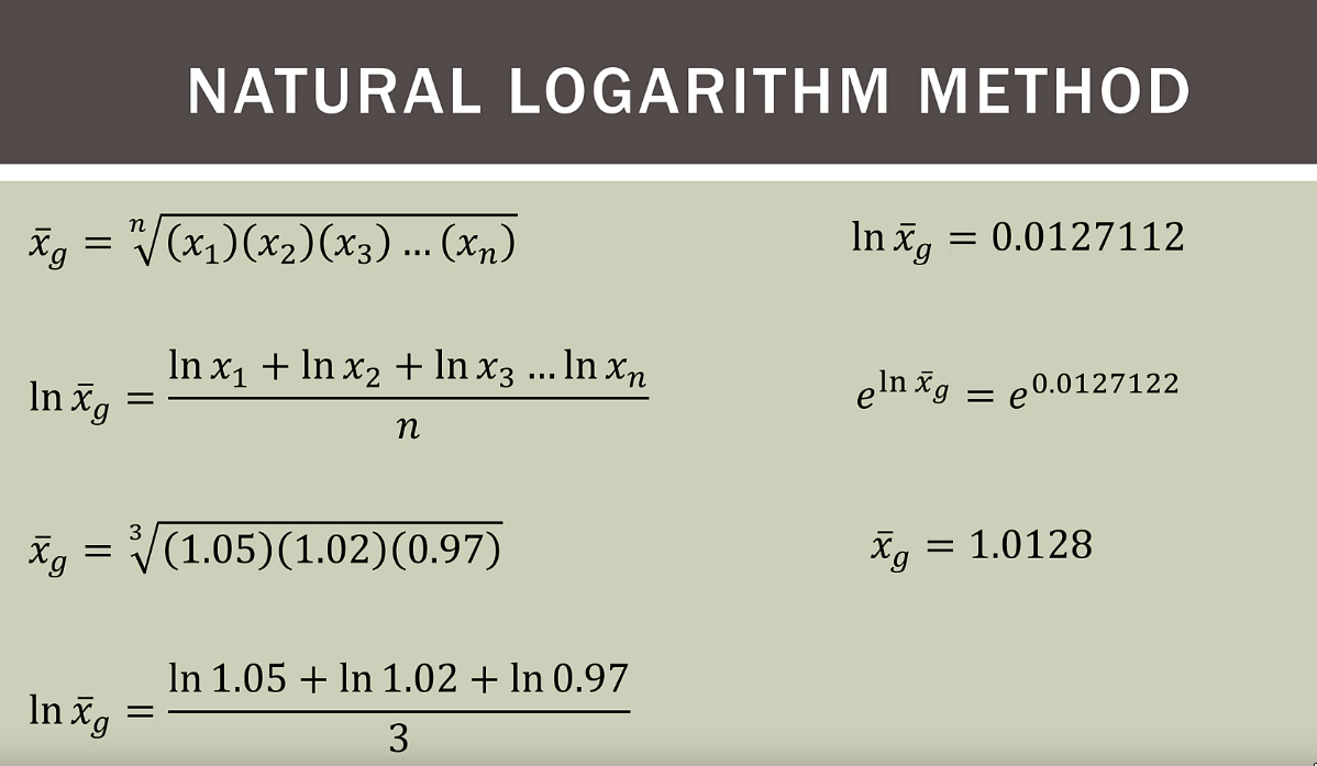
Geometric Mean
- Useful for multiplicative processes
- Useful w Growth rates because they depend on multiplication and not in addition
Median
sortdata inincorderoddobservations: middle value of data arrayevenobservations:meanof the2middle values of data array
Mode
- Observation that
occurs the most - Dataset can have one, multiple or no modes
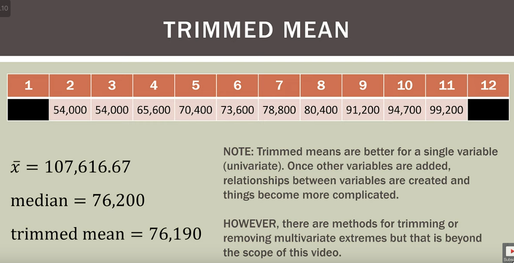
Median vs Mean
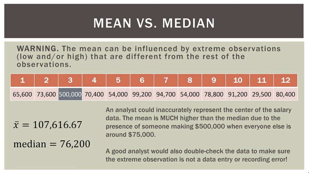 Solution can be Trimmed Mean
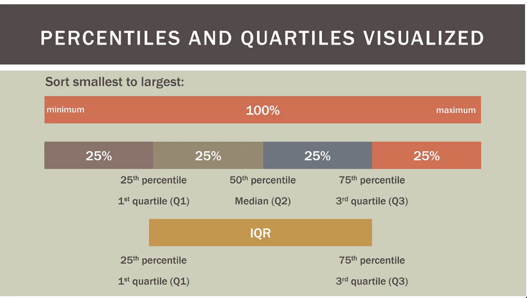
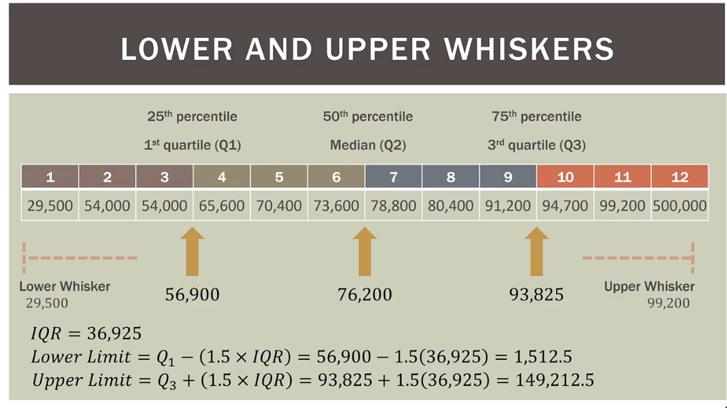
Percentiles, Quartiles(4), Quintiles(5), & Deciles(10)
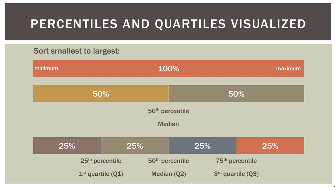
- These just help us locate an observation in a
sorted (low to max)dataset; an address- Doesn’t have to a value in the dataset.
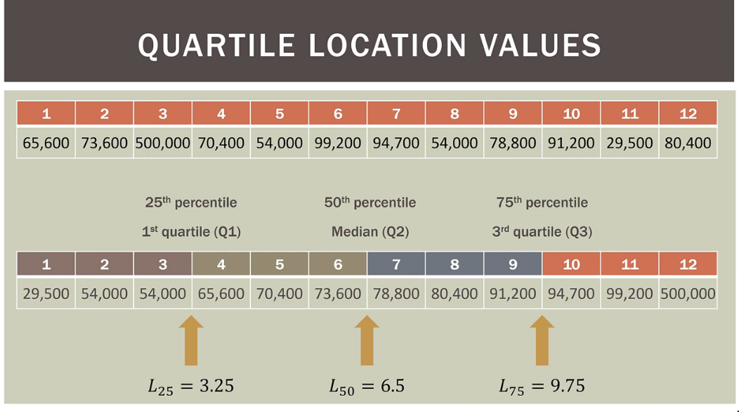
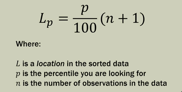
- There’s a location formula, we can calculate the actual value of the percentile from the location even if the address doesn’t point to a data point
- Doesn’t have to a value in the dataset.
- Quartiles, Quintiles, & Deciles are variants of
percetile Percentiles- The
number of values out of the totalthat are at or below that percentile - The observations lie below the said
percentileor above the saidpercentile
- The
- Formula to find
percentilefor some data point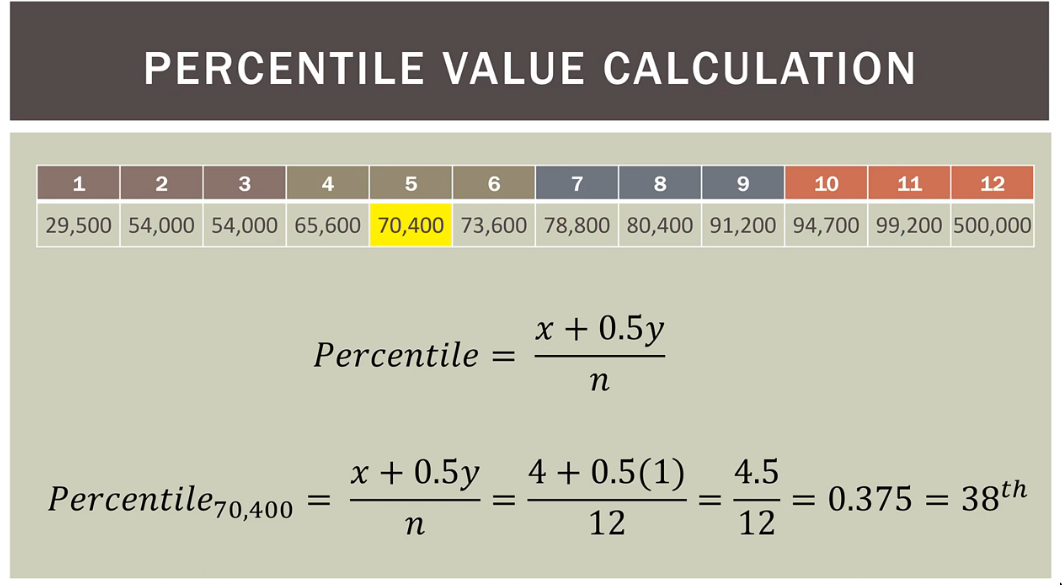
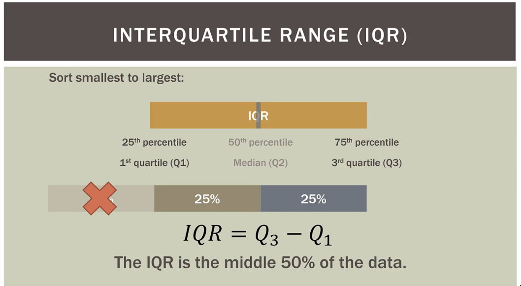
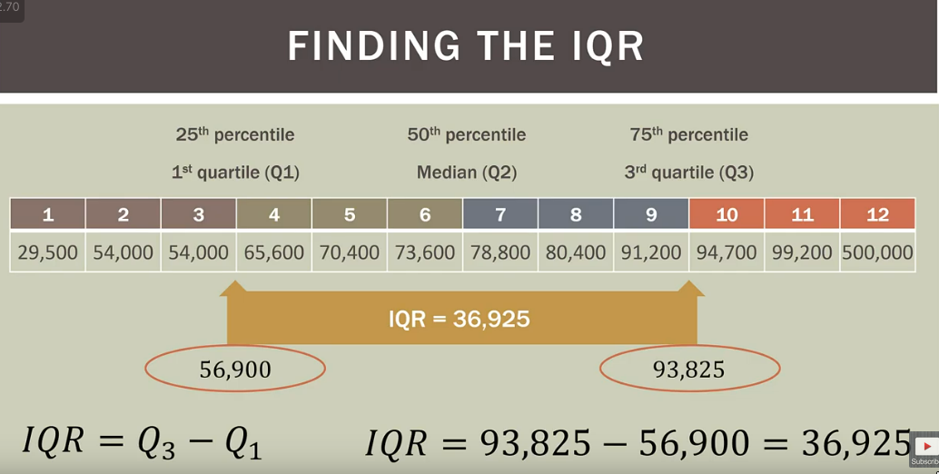
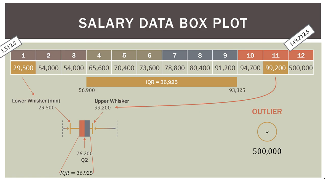
IQR (Inter Quartile(4) Range)
The median will lie somewhere in between the IQR
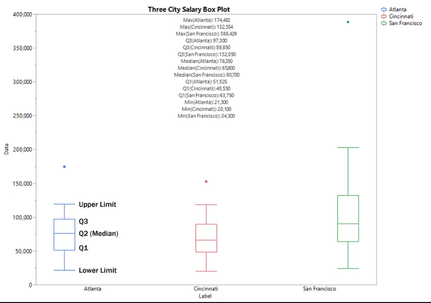
Variability
- Useful when comparing datasets
- Related to the
mean - If things are “spread out”
- Variability answers, “How far is
eachdata point from the mean? (DISTANCE)”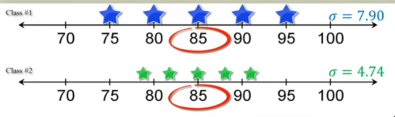
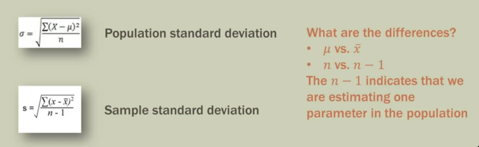
Standard Deviation
Standard Deviationis just thepositive square rootof thevariance- SD is the sqrt of the
sum ofthesquareof thedifference of the data point and the meandivided by theno. of observations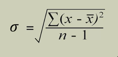
- SD has the convenience of being expressed in units of the original variable. Which is not the case with variance.
- SD is the sqrt of the
- What it says?
- If most data points are close to the mean, variance & SD will be lower
- If most data points are further to the mean(spread out), variance & SD will be higher
Z-score
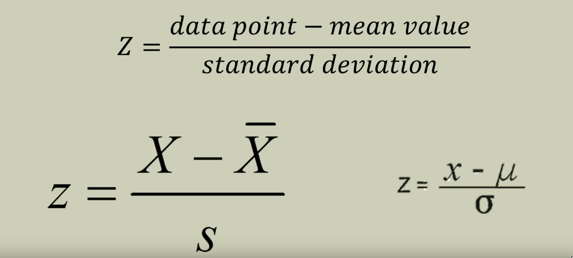
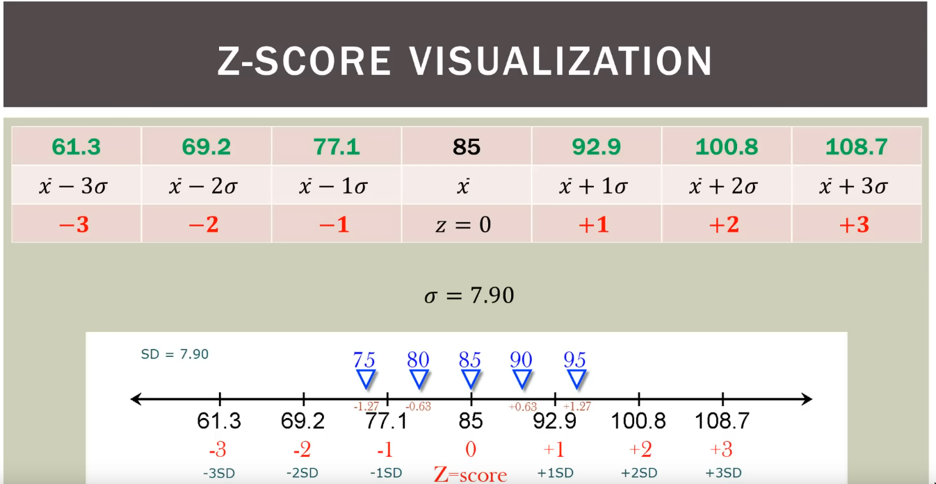
- Z-score answers: “How far is
anygiven data point from the mean? (DISTANCE)”- How many SD away from the mean? (It measures distance in the unit of
sdand ignores any original units such as inches/hours etc.)
- How many SD away from the mean? (It measures distance in the unit of
- The
Z-scorefor themeanitself is0because, it’s0distance away from themean
Bi-variance
Relationship between two variables
-
Covariance
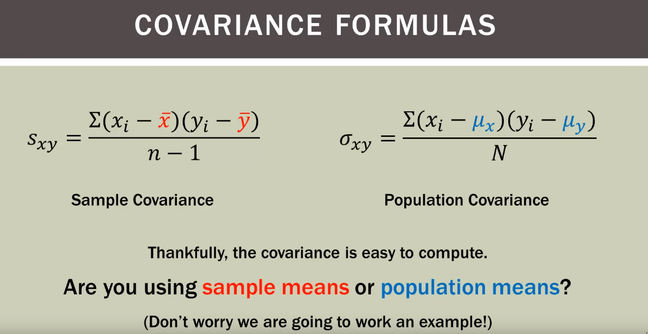
- Shows the
linearassociation btwn 2 variables. - It shows the
direction, not thestrength+ve: increasing linear relation-ve: decreasing linear relation
- No upper/lower bounds, scale depends on variables
- Covariance Matrix
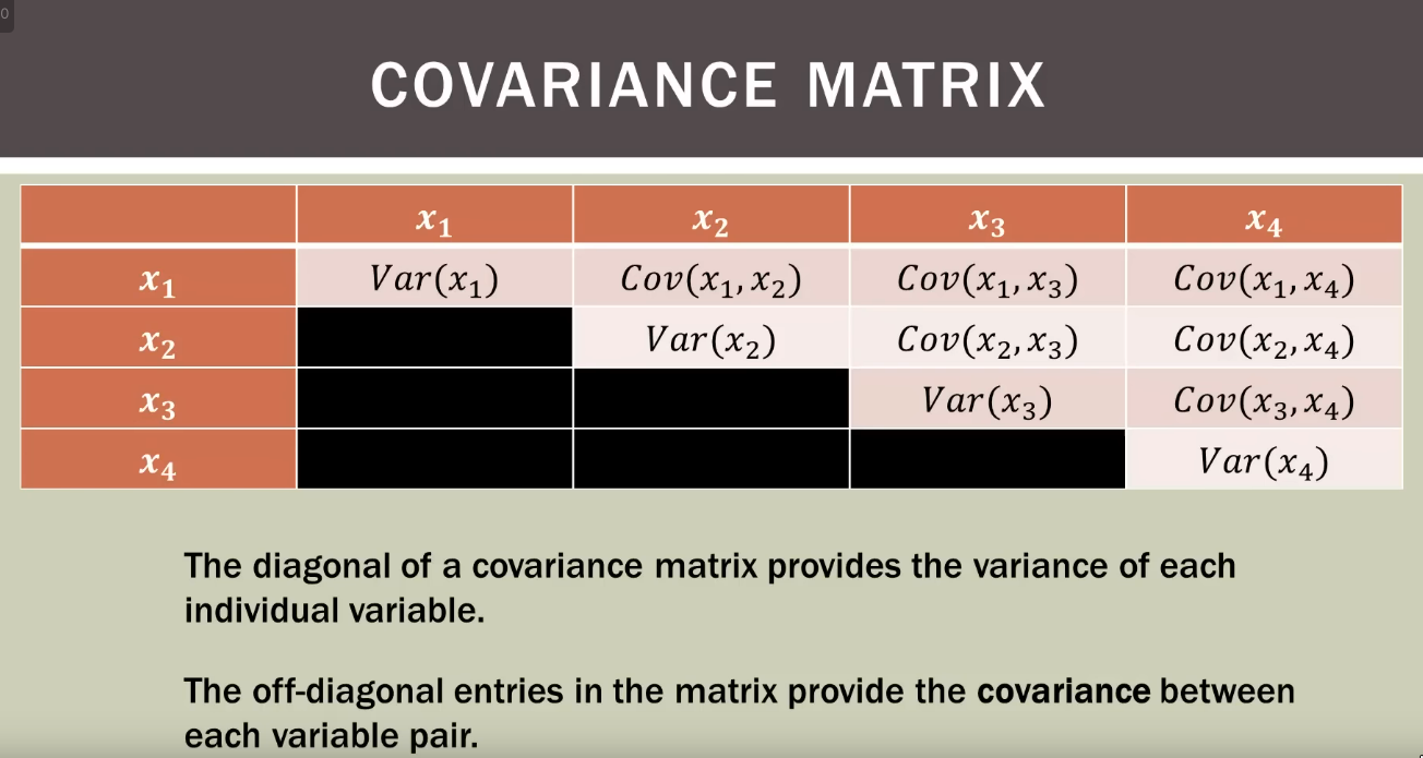
- Shows the
-
Correlation
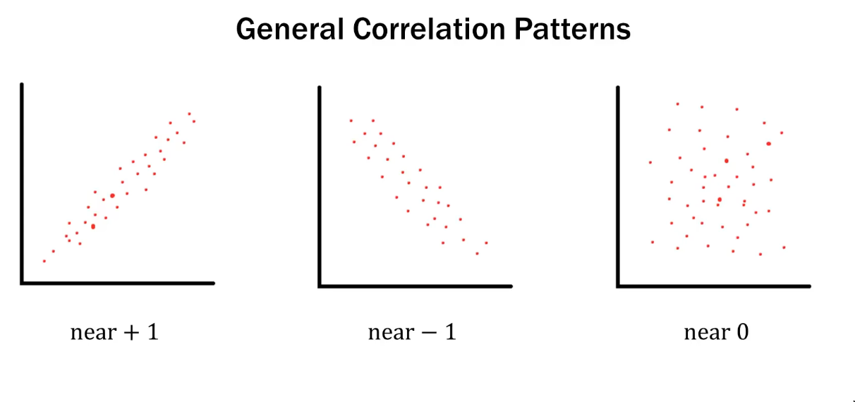
- It shows the
direction, AND thestrengthstrengthof correlation does not mean the correlation is statically significant
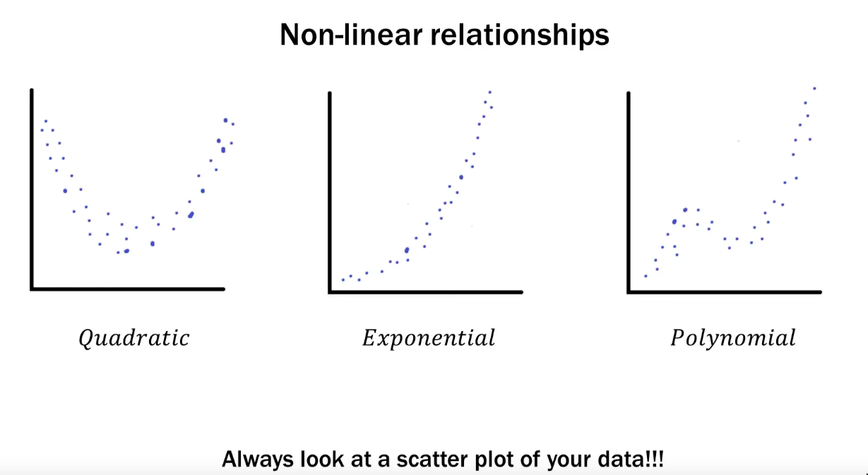
- Only applicable to linear relations
- Always between
-1and1, i.e scale is independent of the scale of the variables - Covariance is not standarized, correlation is standarized. i.e we can use correlation to compare two data sets using different units etc.
- It shows the
- Linear Regression
-
Non Linear data
Hypothesis testing
Bayesian approach
Process
- Unlike frequentist approach, result is not an
actionbutcredible intervals credible intervals: 2 numbers which are interpreted as, “I believe the answer lives between here and here”
TODO Null Models?
Frequentist approach (classical)
“Traditional null hypothesis significance testing and related ideas. These ideas have been under attack for decades, most recently as being one cause of the scientific replicability problem.” - Some user on the orange site
Process
- See good walkthrough of the process
- As a frequentist you don’t believe in anything before analyzing
- Always start with
actioninstead of thehypothesis Step 1: Write down thedefault action- Default action is your cozy place. Incorrectly leaving it should be more painful than incorrectly sticking to it.
- This is the action we choose
- If we know nothing about the data
- If we know partial things about the data (This is usually when we do inference)
- If the result of the analysis falls in the bucket of
null hypothesis (H0)
Step 2: Write down thealternative action- This is the action we choose
- If the result of the analysis falls in the bucket of
alternative hypothesis (H1)i.e not inH0
- If the result of the analysis falls in the bucket of
- This is the action we choose
Step 3: Describe thenull hypothesis(h0)Step 4: Describe thealternative hypothesis(h1)
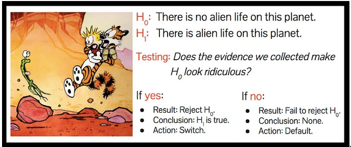
Null Hypothesis
- It is a set of possibilities
- Null hypothesis describes the full collection of universes in which you’d happily choose your default action.
- After the analysis, if
h0isaccepted, we’ve learned nothing interesting. and that’s alright. We do thedefault action - The hypothesis that there is no difference between things is called the Null Hypothesis.
- The hypothesis:
there is no difference - The test: We look for in the data if it convinces us to
rejectthe hypothesis. i.e “Does the evidence that we collected make our null hypothesis look ridiculous?”. This is wherep-valuecomes in.
- The hypothesis:
Null hypothesis (H0)is the mathematical compliment of theAlternative hypothesis (H1). i.e there’s no 3rd bucket- Used to check if two things are different without using any preliminary data/test/experiment
p-value, significance level and confidence interval
- When looking at the result of the analysis to check if the result can be accepted/rejected for the
H0, we usep-value/confidence intervaletc. - Lower
p-value=> more further fromH0 confidence interval- the best guess is always in there
- it’s narrower when there’s more data.
Mistakes / Errors
These are again specific to frequentist stats
-
Type I
- Convicting an innocent person
-
Type II
- Failing to convict a guilty person
TODO Statistical Lies
- People mistake p-values for p(hypothesis|data), mistake p-values for effect size (“it’s highly significant!”); moreover, people using NHST don’t understand multiplicity or “topping-off” problems.