tags : Automata Theory, Algorithms, Computation and Computer Theory
I don’t think I’ve been more confused in my entire fucking life.
- me, 24th April’23
- me, 25th April’23
- Things that I am seeing
- “because people define whatever they please, then the field grows organically, and some things are used more than others”

This page covers what this wikipedia page covers. (Also see, TCS). This is mostly copy paste material, I tried linking back to source when possible, did not want to overload with links as personal note. I am pretty sure info here is incorrect in many places but this is what I understand of it right now.
- 1965 : P was introduced
- Cook & Levin & Karp
Some History
- See
1837
1933
Kurt Godel, Hilbert did something something
1936
Alonzo Church came up with Lambda calculus
1936
- Alan turing came up w Turing machine
- Introduced the idea of decidability
1943
- McCulloch and Walter Pitts presented idea of FSM
- See Automata Theory
1951
- The equivalence of the
regular expressionsandFinite Automatais known as the Kleene’s theorem. - Stephen Kleene described regular languages and regular expressions using mathematical notation called regular sets
- Kleene’s Theorem (CS 2800, Spring 2017)
- ECE374-B SP23: Lecture 5 - DFA/NFA/RegEx equivalence and grammars
- From RE To Automaton : Kleene’s Theorem (a): from regex to automaton
- From Automaton To RE : Kleene’s Theorem (b): from automaton to regex
1956
1959
- Nondeterministic finite automaton was introduced (NFA/NDFA)
- Showed the equivalence to DFA
1965
- Introduced the idea of
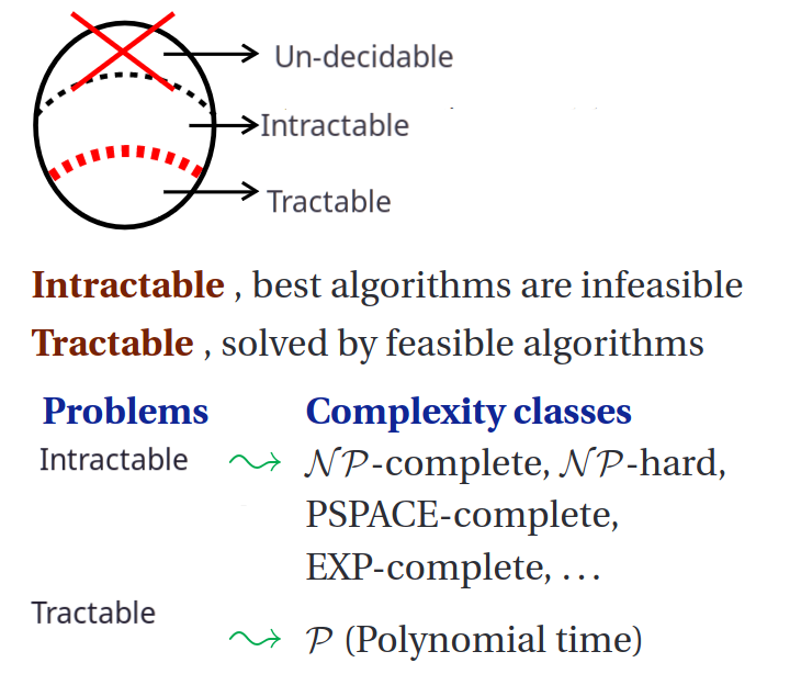
P - Introduced the idea of tractable vs intractable problems.
- Set the stage for
P = NP? - Cobham’s thesis - Wikipedia
1968
- Ken Thompson made Regular Expressions popular by using them in
- Pattern Matching (String Search)
- Lexical Analysis (Scanners, Tokenizer Modules in parsing programming languages)
- For implementing, he used NFA.
- Thompson’s construction (the algorithm) compiled a regular expression into an NFA
- NFA can be converted into RE using Kleene’s algorithm
1970
- was popularized in computer science by Donald Kunuth
1971-1973
- Cook & Levin came up with the proof of existence of NP-complete problems with SAT
- Karp came w more stuff, presented a general framework for proving NP-completeness
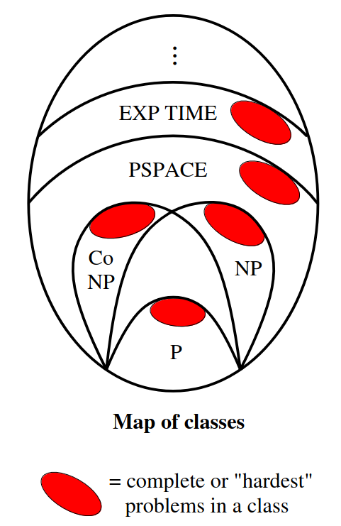
P=NP?was set in discussions.- Meyer and Stock meyer introduced Polynomial hierarchy, introduced
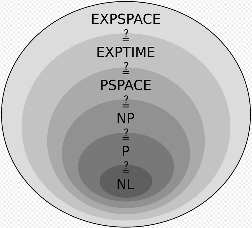
PSPACE
FAQ
You can read the FAQ before reading anything or after reading everything or anytime in between. Basically information in the FAQ is not ordered.
Meta
Computational complexity vs Complexity class
- An
algorithmhas atime/space complexity(computational complexity) - A
problembelongs to acomplexity class.problemsdon’t have run-times.- If you ever come across a discussion discussing time complexity of a problem, it’s probably shorthand referring to the time complexity of the best known algorithm that solves the problem.
P,NP,PSPACE,EXPTIMEetc. are all complexity classes. This means they contain problems, not algorithms.
Can turing machine only solve decision problems?
In practice, are all intractable problems in-feasible and all tractable solutions feasible?
- Here theory and practice differ
- By definition, problems in
Pclass are tractable, but in practice, even n3 or n2 algorithms are often impractical on realistic sizes of problems. (i.e We’d call a problem with a n3 solution to belong inP) - A polynomial-time solution with large degree or large leading coefficient grows quickly, and may be impractical for practical size problems
- Conversely, an exponential-time solution that grows slowly may be practical on realistic input
- A solution that takes a long time in the worst case may take a short time in most cases or the average case, and thus still be practical.
- Saying that a problem is not in P does not imply that all large cases of the problem are hard or even that most of them are.
- Similarly, a polynomial time algorithm is not always practical. If its running time is, say, n15, it is unreasonable to consider it efficient and it is still useless except on small instances.
Is halting problem the end all be all?
NPH & NPC
NP-hard has anything to do with decidability?
- No. Whether a problem is decidable is orthogonal to the hardness.
- NPH + decidable + NP: NPC problems basically
- NPH + undecidable : HALT (Halting problem)
- NPH + decidable + (not) NP : TQBF
Are any NP-complete problems solved in P time?
- No. This would mean P=NP
- But some problems like, 2SAT, XORSAT, Maximum Matching, and Linear Programming, these “seem like they should be NP-complete” at first glance, but then turn out to have clever polynomial-time algorithms.
Are all NP-Hard problems equally hard?
- No. Not all, some are.
- “Equally hard” here means can be reduced to one another.
- Some NP-hard problems may have efficient approximation algorithms that can find solutions that are close to optimal, while others may have no known efficient algorithms or even be proven to be unsolvable in polynomial time.
- Why?
- Every
NPandPproblem is reducible toNP-completeandNP-hardby definition - Any
NP-hardproblem is NOT reducible to any otherNP-hardproblem. - Any
NP-completeproblem can be reduced to any otherNP-completeproblem. - All
NP-completeproblems can be reduced toNP-hardproblems. - So some
NP-hardproblems (which areNP-complete) can be reduced to one another.
- Every
Are all NP-Complete problems equally hard?
- Yes, in a fundamental sense.
- Any
NP-completeproblem can be reduced to any otherNP-completeproblem.
Decision problems
Why are decision problems so popular?
- We focus on studying the decision problems in undergrad complexity theory courses because they are simpler and also questions about many other kinds of computations problems can be reduced to questions about decision problems.
- Most discussions online on complexity classes will be referring to decision problems because
PandNPare classes which contain only decision problems and most discussions online are aboutPandNP. See FAQ for more details on this. - NP-Hardness “officially” is a category of decision problems but people use it for other types of problems too.
- Why are decision problems commonly used in complexity theory?
- complexity of decision problems vs computing functions
What about decision version/counter parts of problems?
- Things can be converted into decision problem easily, which is a good thing.
- Does every computational problem have a decision version?
Why does NP only deal with decision problems?
- First of all, it’s a class of decision problems. So sort of by definition. There are other NP equivalent classes for other types of problems, such as FNP.
- Secondly, verification in polynomial time only makes sense for decision problems.
- You cannot verify an optimization problem in polynomial time because to verify that solution is infact the most optimal, you’ll have to check all solutions and number of solutions can grow exponentially.
Misc
What kind of computational problem is sorting?
- We cannot say it is in
Pbecause sorting is not a decision problem. It can have a decision version of it though. - It seems like a function problem and should belong to
FPcomplexity class but different people have different answers.
TODO What are Lower & Upper bounds for problems & solutions?
- when talking about problems, we are talking about the best known solution, and for the problem it is the worst case. so a problem if stated has a non-poly solution, the algo itself is talking of worst case, so algo might perform 👍 good in better cases
- When we say “NP-complete is hard”
- We’re talking about worst-case complexity
- The average-case complexity is often much more tractable.
Computing model
Turing machines(TM) for describing complexity classes
- If you look into definitions of any of the complexity classes(eg.
P,NP) in this page, you’ll notice that the definitions are based on TM. - There’s nothing problematic about using TM to talk about complexity classes, but its usually implied and I just wanted to be explicit about it.
- Why specifically, TM? My wild guess is because it’s the closest model to real world computing that we do and the foundational work was done relating back to TM.
Computing models other than TM
- There are other models of computations like Lambda calculus, but in general, when we are talking complexity classes, discussions usually are in terms of the TM and related terms.
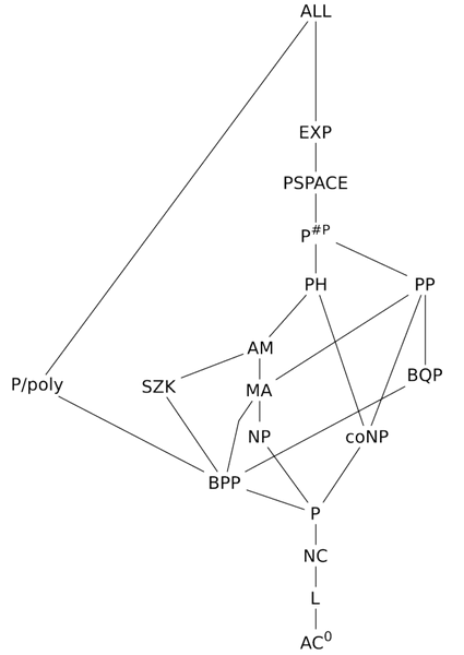
- There are complexity classes for other models of computing, like for Quantum Computer (BQP) and attempts with lambda calculus.
- To be aware of: When we see lower bounds for problems, it’s often given for a model of computation that is more restricted than the set of operations that you could use in practice and therefore there are algorithms that are faster than what would naively be thought possible.
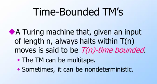
Time Bounded TM
- See Automata Theory
NMT (Nondeterministic Turing Machine)
- This is a thought experiment, this machine does not exist fr.
- NTM that can create parallel timelines and try a different choice in each timeline.
- It can solve NP problems in polynomial time
- If you can
check/verifya solution of length N in polynomial time, just branch on every single possible input of length N. - If you can solve a problem with branching, have the NTM also track the history of every step. Then a valid solution will also have a linear set of steps.
Problem
Formalism of a problem
Language
is the encoding of an input to problem , and the answer to input for problem is “Yes” }
- A
languageis the formal realization of aproblem. languagesare defined by set ofstrings- Each
stringin thelanguageencodes someinstanceof theproblem stringsare defined by sequence ofsymbols- Set of
symbolsis defined by thealphabet - Eg. is the set of all binary sequences of any length.
- Determining if the answer for an input to a decision problem is “yes” is equivalent to determining whether an encoding of that input over an alphabet is in the corresponding language.
- A
stringis in alanguageiff the answer to theinstanceis “yes” - each
stringis the input
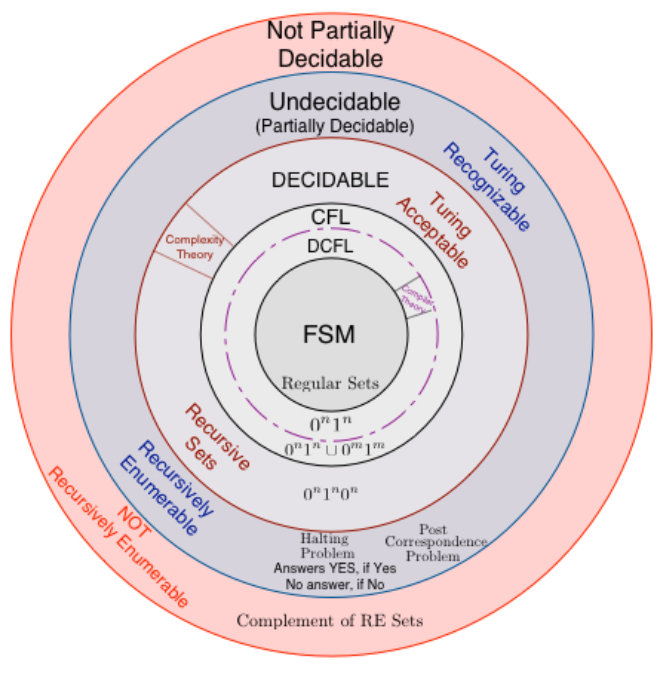
Categorization
These categorizations can overlaps as required.
- Decidability
- Intractability
- Computational work
- Complexity Classes
- Hardness/Completeness (optional)
Decidability
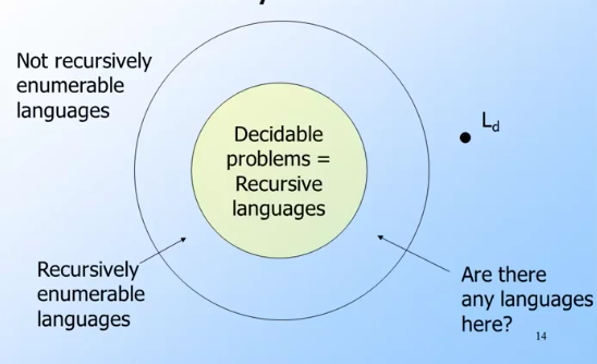
- A problem is said to be decidable if there exists an algorithm with accepts all the elements of and rejects those which do not belong to .
- Time not a constraint when it comes to decidability. If one is able to write any algorithm that does the job, the problem will be decidable.
- Related readings
Intractability
- Again, must remind that it’s a property of a problem and not the solution. But the property itself depends on what solution we have for the problem.
- While decidability was about whether an algorithm for the problem exists or not, intractability is about if the problem has an efficient solution.
- For a more formal definition, see Cobham’s thesis
Computational work
- These are technically called computational problems
- We have categorized problems based on what kind of computational work it requires to get to a solution.
Example computational problem types
- Common ones: decision, search, counting, optimization, function, promise etc.
- More complicated ones: NPO, optimization problems with decision counterparts in
NP. When we say some optimization problem is NP-hard, what we actually mean is that the corresponding decision problem is NP-hard(i.e NP-complete).
Computational problem and their complexity classes
Different computational problems have different complexity classes.
- Decision problems have their own class P, NP etc.
- Function problems have their own class FP, FNP etc. (Natural generalization of
NP) - And so on.
Complexity classes
- Our motive with complexity classes is that we want to put problems of a similar complexity into the same class
- Every complexity class is a
setof formallanguages(problems) - Now because we know that, “Okay, problem X belongs to the same class as problem Y”, we can probably try similar approaches to problem solving that worked for Y.
P
- Contains decision problems
- Problems in this class can be solved in polynomial time or less by a DTM.
- Other names: PTIME/DTIME, Deterministic polynomial class
NP
- Contains decision problems
- Definition 1: Problems that can be
verifiedin polynomial time but may take super-polynomial time tosolveusing a DTM.- Eg. easy to check/verify if a key works, but finding(solve) the right key could take a very long time
- Definition 2: If you had a NTM, this problem are also
solvablein polynomial time.solvablehere means getting anYES - Other names: NPTIME, Non-deterministic polynomial class
co-NP
- Contains decision problems
- Opposite of NP
- It looks for and
NO, if we find aNOthat means it is solvable in polynomial time. - Whether the complexity classes
NPandco-NPare different is also an open question. General consensus is that,NP != co-NP, but there’s no proof.
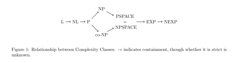
Relationship between complexity classes
- Is there any relationship between time complexity and space complexity
- Why does space(n) <= time(n) imply that TIME(f(n)) is a subset of SPACE(f(n))?
More info
Hardness and completeness
- Hardness/Completeness are properties of a problem that we can “prove” if there is a need to.
- This is just another further categorization of problems which tries to specify a relative hardness to problem.
- Here we’re talking in general sense, we’re not talking about NP-hard or NP-complete, just the general idea of hardness and completeness.
What does being “hard” even mean?
- Again, I’ll re-specify that hardness is a property of a problem and not a property of a solution(algorithm).
efficient/inefficient: Terms used withalgorithmseasy/hard: Terms used withproblems
- Well, “hard” does not really mean “hard”. WTF?
- What I mean is, what’s hard for a computer may not be hard for a human. And what’s hard for a human may not be hard for a computer. In-fact, there are lot of “efficient” solutions to “hard” problems.
- So we’re talking in terms of hardness for computational problem that a computer will compute. With some loss of generality, we can say “easy problems” are the ones that are solved in polynomial time and “hard problems” are the ones that take superpolynomial(more than polynomial) time.
- It’s similar to how time-complexity(in the world of algorithms) has nothing to with how complex it is to understand an algorithm. An algorithm might be really simple to understand for you but might have a time complexity of .
- These 2 blog-posts do a better job at explain the idea of why NP-Hard problems are not really hard.
General idea
- I have this problem
Xthat I am not able to solve. - I know there’s problem
Ythat is not solved by humanity yet. - If I can somehow prove,
Xis as hard asY, I can now not worry about solvingXefficiently and look for other approaches that were taken to solveY, and maybe it’ll work for my problem. - This “proving” is what it takes to make something to be
hard/complete, a problem by itself does not becomehard/complete
Hardness vs Completeness
 Both of these property are always relative to some existing complexity class. Eg.
 X-hard, X-complete (Where X is some complexity class), NP-hard, NP-complete, P-complete and so on.
- Hardness
- If something is
X-hardit is at least as hard as the hardest problems in class. - So if we call something
X-hard, that means it may even belong outside the classX. - If something is NP-hard, it could be even harder than the hardest problems in NP
- If something is
- Completeness
- If something is
X-completeit is among the hardest problems in that class. - All
X-completeproblem will belong to the classX - {
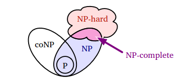
X-completeproblems } is a proper subset of {X-hardproblems }
- If something is
NP-hardness & NP-completeness
Before understanding NP-hardness and NP-completeness, you should understand what NP is(a complexity class, what it means to be a complexity class), and you should understand the terms “hardness” and “completeness” in general sense.
A bit of history (1970s)
Cook, Levin and Karp cooked something
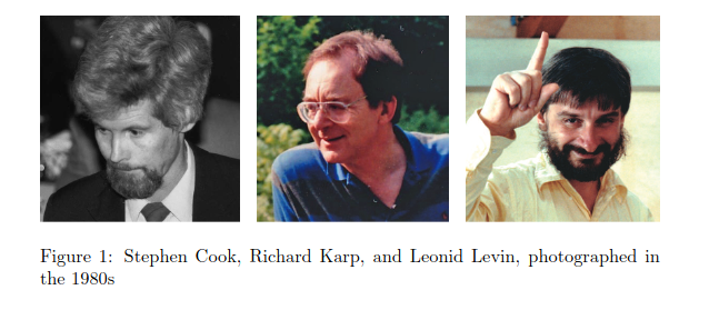
- Cook and Levin said that SAT problem is
NP-complete.- SAT was the first problem to be proven
NP-complete. - i.e Any problem in
NPcan be reduced in polynomial time to SAT. - i.e If SAT is solved, all
NPproblems will be solved in polynomial-time. If this happens,P=NP.
- SAT was the first problem to be proven
- Around the same time, Karp showed that 21 diverse combinatorial and graph theoretical problems, each infamous for its intractability, are NP-complete
How does their help?
I mean it should not be a question at this point but it helps in 2 ways that I can think of.
- It helps to show that your problem is infact hard
- Before proving SAT is
NP-complete, there was no reference to a truly hard problem, so this allowed us to define hardness. - If prove your problem to be NP-complete, then you have tied its hardness to the hardness of hundreds of other problems.
- Your problem is now at-least as hard as the hardest NP-complete problem.
- So now you can stop looking for an efficient solution because there exists none.
- Before proving SAT is
- If ever
P=NP, we have a way to solve every problem inNPin polynomial time with a DTM.- For any NP-problem , there is a polytime algorithm α reducing SAT to . (by def.)
- Take an instance of , turn it into an instance of SAT via α
- Now this is where our current world is at. ⏲
- If we ever find a polynomial-time solution for SAT, say β
- Now we can use β to solve because we reduced SAT to
- Since reduction algorithm(α) was polynomial time, final solution is polynomial time.
Reductions
- There is a general idea of reduction, but we’ll focus on reduction wrt
problems - Reductions are “algorithms” that converting one problem to another.
- Reduction is a systematic way to transform instances of one problem into instances of another, so that solutions to the latter translate back to solutions to the former.
Cook’s reduction
- AKA Turning reduction
- AKA Polynomial-time reduction
- Allows you to call the black-box more than once.
Lis NP-hard if- For any decision problem
BinNP Bcan besolvedinPtime by a TM with oracle access toL.
- For any decision problem
Karp’s reduction
- AKA Many-one reduction
- Allows you to call the black-box problem exactly once. (I don’t really understand this part)
Lis NP-hard if- For any decision problem
BinNP Bcan betransformedinto an instance ofLinPtime using a TM.
- For any decision problem
TODO Direction of reduction
- To prove a
Xis hard: Reduce toX - Clarification on the reductions
- When we reduce to , we are saying that is at least as hard as . But could be easier.
- When we try to prove hardness, we reduce
fromthe known problemtothe problem we’re trying to prove- i.e Reduce from SAT to
X. Now we knowXis atleast as hard as SAT. - i.e Reduce Halting to
X. Now you can try reducing this but you most probably won’t be able to because halting is probably harder than your problem.
- i.e Reduce from SAT to
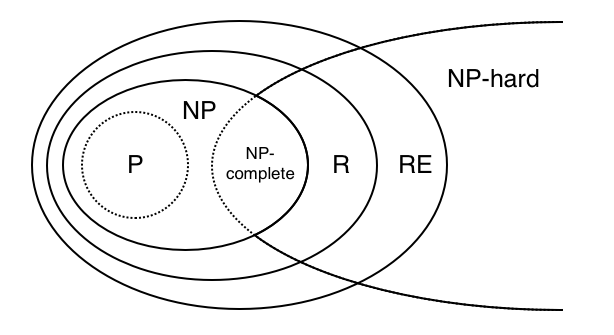
NP-hard & NP-complete
NP-hard (NPH)
- Hardness itself is not specific to decision problems. But
NP-hardnessis specific to decision problems but sometimes used for other computational problems as-well depending on context. - Based on the reduction used(Cook v/s Karp),
NP-hardwill have a slightly different meaning. Most discussions will be referring to Karp’s reduction though. - Problems in this class do not have to be a decision problem
- The definition following will be based on Karp’s reduction.
- If each
NPproblem can be reduced(in poly-time) to a problemL. ThenLcan be consideredNP-hard
NP-complete (NPC)
- Decision problems which contains the hardest problems in
NP NP-completeproblems is a proper subset ofNP-hardproblems.- As a general rule, if it is in
NPand it is not known to be inP, then it’sNP-complete. AssumingP != NP, exceptions go in NP-intermediate - There are a lot of lists on the internet with NP-complete problems.
Difference between NP-hard and NP-complete
Solution
Formalism
Algorithm: A Turing Machine is the formal analogue of an algorithm. Algorithm is the TM.
How is it represented?
- We want to represent the asymptotic behavior of the algorithm, the function. For this, we use Big Oh Notation (See big-o growth)
- A language to talk about functions
- We’re just talking about properties of functions, we’re not talking about meanings.
Computational complexity
- Complexity is the number of operations.
- It is a relative measure of how many steps it will need to take to achieve something wrt to the input length.
- It has nothing to do with how long it is to write down the solution or how complicated it is to follow.
Time complexity
Space complexity
Analysis
Relationship of Complexity Analysis and Big Oh
- In algorithm complexity analysis we’re more interested in bounds of Big Oh Notation
- The statement “X case is ”, for any values of
X,Y, ,f,nis valid. Eg. Nothing is stopping you from saying “The best case is ” or “The worst case is ”. That is, the bounds do not relate to the case, it’s only after the analysis we can say something about it. - In practice, we mostly talk about worst case in terms of upper bound however.
Types of Analysis
Lot of analysis we can run by using Big Oh Notation
- worst-case running time (most common)
- average-case analysis
- best-case analysis
- expected time analysis for randomized algorithms
- amortized time analysis, and many others.
Asymptotic Analysis
- Asymptotic complexity simply talks of individual (worst) cases. The measure is against the size of input only—not against the data and/or operations (probability) distribution over many executions
Amortized Analysis
- Amortised complexity of an algorithm is expressed as the average complexity over many (formally infinite number of) cases.
- The idea is that if you run certain operations very many times, and in the great majority, the operations run very fast (e.g. in constant time), it’s OK that in some rather rare cases, they run for quite a long time; these cases are made up for (i.e. amortised) by all the other fast cases. It makes sense to compare algorithms using amortised complexity analysis if you expect them to run very many times and the you’re only seeking the whole to be efficient, not the particular runs.
Cases
- A
casefor an algorithm is associated with an instance of a problem. More precisely the “inputs”. - We have: Best, Worst and Average case (WCRT, ACRT, BCRT)
Graph for a function/algorithm
For any function(algorithm)
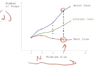
- We have a
Time v/s Sizegraph of WCRT,ACRT and BCRT - Each dot represent different variation of the same input size(eg. sorting [1234] vs [4321])
Average case (ACRT)
- BCRT and WCRT are apparent.
- ACRT is picking cases at random
- Randomized algorithms are getting popular, those algorithms usually require ACRT analysis to show merits
WCRT is vs WCRT is
- Sometimes we can make exact statements about the rate of growth of that function, sometimes we want to express upper or lower bounds on it.
- Not all algorithms can have complexity. There are algorithms that vary in complexity. Those can only be described with Big-O complexity
- When we say , the function may also be , we do not know.
- When we say , we know for a fact the function is and , because it is bounded by
- When we say will be lower-bounded by and upper-bounded by , we know and
- Therefore we can say that gives us a more accurate (or at least equal) sense of worst-case run time than
Upper and lower bounds
Proving hardness and reducing
For NP
- You don’t really prove hardness for NP because NP itself says nothing about hardness. But you can prove membership.
- It’s just a class of decision problems that gets verified in polynomial time.
- But to prove NP membership, you can just use the solution as the certificate to state that it’s in NP. But the certificate needs to be polynomial time, i.e you should be able to verify it in polynomial time.
- Two ways
- Actually describe a non-deterministic polynomial algorithm that solves the problem.
- Use a certificate and verifier approach
- Proof that this problem is in NP
For NP-hard
I have lost my patience dealing w this topic. This section might contain incorrect info.
- It’s generally not apparent if a problem is NP-hard or no. So we need to prove it.
- When we say “we need to prove hardness”, this is what we mean.
- While trying to prove that
LisNP-hardwe need to reduce an existingNP-hardtoL. - It’s a prerequisite to proving
NP-complete, asNP-completeis a proper subset ofNP-hard. - We can probably prove something is
NP-harddirectly, but commonly we usereduction. - There’s a library of NP-hard problems that you can pick from, some of them are cleverly designed to be easy to be reduced to. Try to get a feel over time for which problems more easily lend themselves to different schemes, like packing, or covering, or traversing graphs.
- Do a reduction on the problem. If the reduction is same as the reduction of some other known NP-Hard problem, we’re done. The reduction itself should take polynomial time

For NP-complete
- You have to prove membership to
NP- that it is a decison problem
- that it is verifiable in poly-time
- You have to prove membership to
NP-hard - Examples
For NP-hard but not NP-complete
- Proving that a problem is in
NP-hardbut not inNP-completeis tricky - This demands we prove the problem
- Does not exist in
NP - Is harder than any
NP-completeproblem, becauseNP-completeis a subset ofNP-hard
- Does not exist in
- There’s no known way to directly compare the hardness of problems that are not in NP with those that are. We can use approximation.
- Example
- Halting problem
- The optimization-version of traveling salesman where we need to find an actual schedule is harder than the decision-version of traveling salesman where we just need to determine whether a schedule with length <= k exists or not.
For NP-hard but not known to be NP-complete
- Mario was proved to be
NP-hardbut notNP-complete. Here is some explanation that I don’t yet understand.
Dealing with hard problems
- Dealing with
NP-completeproblems andNP-hardproblems is more or less the same asNP-completeproblems areNP-hardas-well. - But not all
NP-hardproblems areNP-complete, but most of these problems have decision problem counter parts that fall inNP-complete. - Once you know a problem is hard(
NP-completeorNP-hard), you can ask, “can I find good approximate solutions?“. Eg. See how Bin packing problem is handled with. It’s bothNP-hardandNP-complete. NPO is the class of optimization problems whose decision versions are in NP - Dealing with intractability: NP-complete problems
- I need to solve an NP-hard problem. Is there hope?
- What is inapproximability of NP-hard problems?
- Is there any NP-hard problem which was proven to be solved in polynomial time?
- How to determine the solution of a problem by looking at its constraints?
P vs NP
The Question
- Q: is
P = NP? - Q: Are
PandNPthe same class? - Q: Can problems which are verified in p-time also be solved in p-time?
- Q: If it’s easy to check the solution, is it also easy to find the solution?
What we know about the question
- What
P,NP,NP-hardandNP-completemean. NPproblems here refers toNP-completeproblems. (VERIFY)Pis a subset ofNP, but not sure if it’s a proper subset.P != NPis currently the general consensus by Computer Scientists- It’s easy to understand for mere mortals too. It’s almost is natural.
- That solving is harder than just checking a solution.
- BUT, No one knows how to prove
P != NP, hence we have this question.
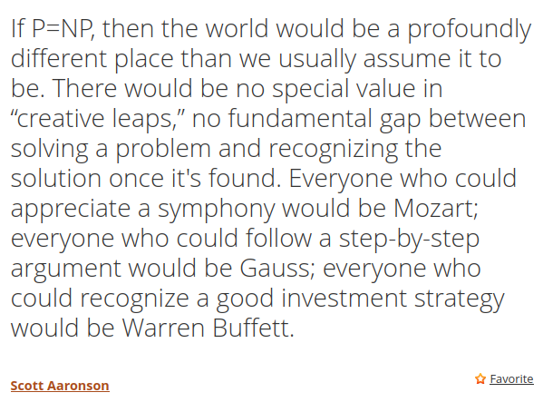
What happens if P = NP?
- Problems which are easy to check will become easy to solve
- It’ll be possible to reduce every
NPproblem toP - It’ll be possible to reduce every
NP-completeproblem toP - For problems that are in
NP-hardonly, it’ll mean nothing.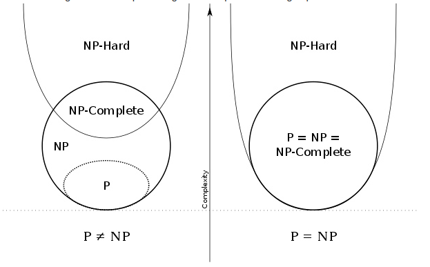
- Public Key Cryptography will be broken.
What happens if P != NP?
- It’ll mean
Pis a proper subset ofNP - Some problems are inherently complex to solve.
NP-hardproblems cannot not be solved in polynomial time.
Resources
- P vs. NP - The Biggest Unsolved Problem in Computer Science - YouTube (Some issues)
- Simon Singh
- NP-Complete isn’t (always) Hard
- 8. NP-Hard and NP-Complete Problems - YouTube (Lot of issues)
- P vs. NP and the Computational Complexity Zoo - YouTube
- Lambda Calculus vs. Turing Machines
- NP-Completeness, Cryptology, and Knapsacks